The Stueckelberg Parameter Space

Move along either axis and you recover the same hidden physics

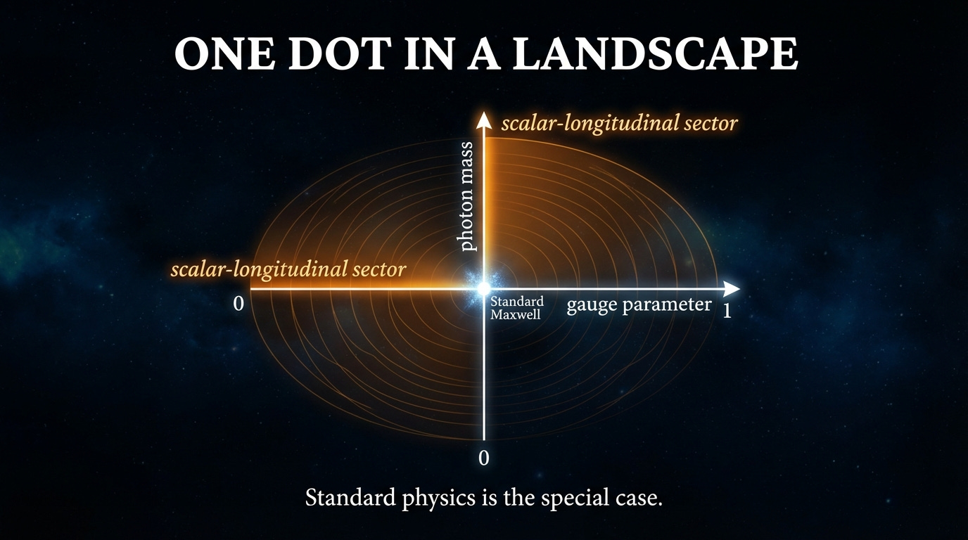
There’s a diagram in my paper that changed how I think about standard electrodynamics. Not because it introduces new physics. Because it shows that standard electrodynamics is a single point in a larger landscape. And both directions away from that point lead to the same place.

---

⬅️ Previous: P = ψψ*. The Born rule uses both time directions in every probability calculation. The “deleted” advanced wave was hiding in the complex conjugate all along.

The Born Rule Contains Both Time Directions

---

The Two Parameters

The Stueckelberg Lagrangian is standard quantum field theory. It’s in the textbooks. It describes an electromagnetic field with two additional parameters beyond what Maxwell’s equations use.

The first parameter is the gauge-fixing parameter γ. In standard electrodynamics, γ functions as a mathematical device: you can set it to any value (Feynman gauge γ = 1, Landau gauge γ → ∞) and all physical observables come out the same. This is the standard story of gauge freedom: γ is “unphysical.”

The second parameter is the Stueckelberg mass m. Give the photon a small mass, and a third polarization state appears: the longitudinal mode. This is the Proca mechanism. The photon mass has an experimental upper bound of m < 10⁻¹⁸ eV/c², which is very small. But “very small” and “exactly zero” are different claims with different physical content.

Standard Maxwell electrodynamics sits at the origin of this parameter space: γ = 1 (conventional gauge fixing) and m = 0 (massless photon). Two transverse polarizations. The familiar theory.

Both Axes Lead to the Same Place

Now do something that nobody in the standard curriculum ever does. Move away from the origin.

Along the mass axis: increase m from zero. The Proca mechanism activates. A longitudinal polarization appears. The photon acquires three polarization states instead of two. The scalar-longitudinal sector opens up.

Along the gauge axis: instead of treating γ as a mathematical device, promote it to a physical parameter. Set γ = 1 in the Stueckelberg Lagrangian. The gauge-fixing term, which was an external constraint, becomes a kinetic term. The Lorenz divergence ∂_μA^μ, which the Lorenz gauge sets to zero, becomes a dynamical field C with its own wave equation: □C = sources.

Different axis. Different mechanism. Same hidden sector.

The mass axis gives you longitudinal modes through the Proca mechanism (adding mass). The gauge axis gives you longitudinal modes through gauge promotion (removing constraints). They arrive at the same physics from opposite directions. The scalar-longitudinal sector isn’t an exotic addition to electrodynamics. It’s what you find in every direction away from the special point where standard electrodynamics sits.

The Convergence Pattern

This two-axis structure explains something that initially seems like a coincidence. Four independent derivations between 2003 and 2020, using different mathematical frameworks, all recovered the same scalar-longitudinal physics:

Van Vlaenderen (2003) approached through gauge-free classical electrodynamics. Hively and Giakos (2012) through extended electrodynamics derived from the Stueckelberg mechanism. Reed and Hively (2020) through systematic gauge relaxation with Woodside’s uniqueness theorems. The Stueckelberg/Proca literature arrived through the mass parameter.

Four derivations. Different starting points. Same destination. The parameter space diagram explains why: there is only one destination to reach. Standard electrodynamics is a special point. Every direction away from it leads to the scalar-longitudinal sector because that sector is the generic case. The four-potential A_μ supports three propagating modes (two transverse plus one scalar-longitudinal). Getting it down to two requires imposing the Lorenz constraint. The constraint is the special case. The three-mode theory is the default.

What the Special Point Hides

Sitting at the origin of the parameter space, standard electrodynamics can’t see three things.

The scalar field C: the Lorenz divergence, which the gauge convention sets to zero. When it’s dynamical, it propagates as a wave with properties distinct from electromagnetic radiation. No magnetic field. Potential-sector penetration of Faraday enclosures (the E-field is screened by charge relaxation, but the potentials pass through). 1/r² attenuation. Monopolar reception. These signatures are invisible at the origin because the field that carries them is constrained to vanish.

The longitudinal force: the Grassmann force law, which underlies the standard Lorentz force, is provably non-reciprocal for open circuits. Newton’s third law is violated whenever ∇·J ≠ 0. Restoring the longitudinal component via the Whittaker force law fixes the symmetry. But the longitudinal component exists only in the scalar-longitudinal sector, which the gauge constraint suppresses.

The energy channel: the generalized Poynting vector in Extended Electrodynamics contains an additional term, -𝐄S, where S is the scalar field. For scalar-longitudinal waves, the standard 𝐄 × 𝐁 Poynting flux vanishes identically. The entire energy flow occurs through the scalar channel. At the origin, this channel doesn’t exist because S is constrained to zero.

The Uniqueness Result

Woodside’s decomposition theorems establish something stronger than “the scalar-longitudinal sector exists.” They establish that the EED decomposition of the electromagnetic field into transverse and scalar-longitudinal components is unique. There is exactly one way to decompose the four-potential into a gauge-invariant transverse part and a gauge-dependent longitudinal-scalar part, given appropriate boundary conditions.

This means the four-derivation convergence isn’t surprising. It’s mathematically necessary. There is only one scalar-longitudinal extension that’s consistent with the symmetry structure of the four-potential. All four derivations found it because it’s the unique answer.

What Standard Physics Does Know

The standard theory isn’t wrong about any of this. It knows the Stueckelberg Lagrangian. It knows the Proca mechanism. It teaches both. What it doesn’t do is take the parameter space seriously as a map of physical possibilities.

The standard curriculum treats γ as a mathematical device and m = 0 as exact. It teaches students to work at the origin and declares the rest of the parameter space unphysical. The evidence, from Aharonov-Bohm through superconductor physics to the dynamical Casimir effect, suggests that physics doesn’t live exclusively at the origin. It’s using the full space.

The parameter diagram doesn’t ask you to accept exotic physics. It asks you to notice that the physics you already accept is a special case of a larger theory you already have.

The full argument, with the Lagrangian, the convergence table, and eight lines of evidence, is in my paper “The Deleted Degrees of Freedom.” Free to read.

https://advanced-rediscovery.com/research/deleted-degrees-of-freedom

The derivations, the full experiment catalog, the three-test discriminator protocol, and the reading list that didn’t fit in these articles — it’s all in The EED Playbook, available for paid subscribers.

---

⏭️ Next: “Scalar-longitudinal waves. You’ve heard claims. Here are answers, with equations, experiments, and sources.” Part 1 of the 100 Questions series. Tuesday.